Can we use Convolutional Neural Network also known as Convnets (CNN) in algorithmic trading? Did you read my post on how to use Facebook Prophet Predictive Algorithm in trading? So can we use Convolutional Networks in algorithmic trading and forex trading? In this post I will answer this question by building a currency price predictive model using CNN. Convolutional Neural Networks (CNNs) have been a breakthrough in the field of image recognition. Important question that comes to mind is can we use these CNNs in algorithmic trading. CNNs are considered to be very advanced. The idea to use CNNs in algorithmic trading came to my mind when I read a research paper downloaded from ResearchGate in which someone from Italy claimed that he achieved above 80% success rate in currency pair price prediction. Deep Learning is the new revolution that has taken over the landscape of Artificial Intelligence. In this post I am going to discuss in detail how we can use deep learning especially Convolutional Neural Network in our trading algorithm If you are new to deep learning, you can take a look my course Deep Learning For Traders. In this course, I take you by hand and show you what is deep learning and how you can apply it to improve your trading.
A Brief Introduction To Convolutional Neural Networks
Convoutional Neural Networks also known as Convnets have made breathtaking breakthroughs in the filed of image recognition and classification. Google has developed a number of advanced convnet architectures that includes that famous 22 layer GoogLeNet. Chinese game Go has been considered to a longtime Artificial Intelligence Challenge. Convolutional Neural Networks have been trained to play the game of Go.Convolutional Networks have achieved success rates between 85% to 90% against top class world players of Go. Keep this in mind. Go is much more demanding game as compared to Chess. This is something important for us. Despite their big success in image recognition convnets are being used in many other demanding artificial intelligence fields.So I believe we can apply convnets to train a financial time series and use that in oour algorithmic trading system. Facebook is also using CNNs in face recognition in its DeepFace program. IBM, Microsoft, Twitter, Baidu and other high tech companies are also using convolutional networks in their artificial intelligence programs. These were the top players in Artificial Intelligence.
You can see Convolutional Neural Networks have been the biggest breakthrough in the filed of deep learning and artificial intelligence with many wide ranging applications. If you are new to deep learning, you can take a look at my course Deep Learning For Traders. In this Deep Learning for Traders course, I teach you in depth about convnets and recurrent neural networks (RNNs) that are ideal of time series forecasting. Long Short Term Memory Networks also known as LSTM networks and Gated Recurrent Units also known as GRUs are important RNNs. There are many people who are selling neural network forecasting software to traders for $1K to $2K. By taking my course you will be able to build your own neural networks for price forecasting and you don’t need to buy any expensive forecasting software. You can read my post on how to use Echo State Neural Networks in forex trading.
As said above Covnets were developed for better image identification. Early neural networks had limited neurons. You should be familiar with artificial neural networks. Artificial neural networks were developed in early 1950s. These artificial neural networks used the human brain neural network model in which billions of neurons are interconnected. In those days computer technology was in its infancy. So interest in artificial neural networks waned very soon. In 1990s when computer technology had become advanced, artificial neural networks again got interested. In 2000s, lot of work was done and the breakthrough came in 2010s when Deep Learning Networks was discovered.
Deep Learning Networks are neural networks with many hidden layers. These hidden layers can run into hundreds and thousands. Computer technology has become sufficiently advanced to train these deep learning networks. As said above Convolutional Neural networks provided the much needed breakthrough with image classification. Google has developed its own deep learning library Tensorflow. We will be using Tensorflow as the backend of our Keras model. Now a little introduction to convolutional neural network architecture:
- Input Layer: This layers takes the raw input data.
- Convolutional Layer: This layer calculated the convolutions between the neurons and the input patches.
- Rectified Linear Unit Layer: This layer applies the RELU activation function to the previous layer.
- Pooling Layer: This layer restructures the output from the previous layer into a lower dimension output.
- Fully Connected Layer; This computes the output in the previous layer.
Modelling High Frequency Data Using Convolutional Neural Network
Modelling high frequency price data is a challenge. High frequency are all intraday timeframes like 1 minute, 5 minute, 15 minute, 30 minute, 60 minute and 240 minute. Daily and weekly timeframes are low frequency data. High frequency price forecasting modelling is very different from low frequency price forecasting modelling. You should keep this in mind that high frequency return data is nor normally distributed. This is an important thing for you to understand. Normal data is 99% within 3 standard deviations from the mean. When the return data is not normally distributed means there can be extreme values that we call outliers. Our high frequency price forecasting model should be able to cater for these extreme values. You can read this post in which I explain in detail how high frequency return data is not normally distributed.
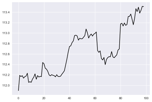
You should have Python installed on your computer. Anaconda allows you to install Python on your computer seamlessly. We will be using Keras library with Tensorflow library as backend. There are a number of brokers that allow you to build algorithmic trading systems using their Python APIs. Below is the plot of the close price that we will use to build the deep learning model.
#Convolutionsal Neural Network For Predicting Price
#import the following modules
from __future__ import print_function   #A
import pandas as pd
import numpy as np
from matplotlib import pyplot as plt
import seaborn as sns
import datetime                         #A

#define the DIFFERENT input variables
train_end=24                            #B
N=24

#Read the dataset into a pandas.DataFrame
data1 = pd.read_csv('D:/MarketData/EURUSD+60.csv',
header=None)
data1.columns=['Date', 'Time', 'Open', 'High',
'Low', 'Close', 'Volume']
data1.shape

#Let's see the first five rows of the DataFrame
data1.head()                              #B

# We need to merge the data and time columns
# convert that column into datetime object
data1['Datetime'] = pd.to_datetime(data1['Date'] \             #C
+ ' ' + data1['Time'])
#rearrange the columnss with Datetime the first
data1=data1[['Datetime', 'Open', 'High',
'Low', 'Close', 'Volume']]                                      #C

data1= data1.iloc[len(data1)-300:len(data1),]                   #D
data1.head()

# we need to scale the close price to [0,1] range

from sklearn.preprocessing import MinMaxScaler                  #E
scaler = MinMaxScaler(feature_range=(0, 1))
data1['scaled_Close'] = scaler.fit_transform(\
    np.array(data1['Close']).reshape(-1, 1))
data1.head()
data1.shape                                                      #E

# divide the data into train set and test set
#We use Keras with Tensorflow backend to train                   #F


df_train = data1.iloc[0:len(data1)-train_end-1,6]
df_val = data1.iloc[len(data1)--train_end-10:len(data1)-train_end,6]
print('Shape of train:', df_train.shape)
print('Shape of test:', df_val.shape)
df_train.tail()
df_val.tail()

#Reset the indices of the validation set
df_val.reset_index(drop=True, inplace=True)
df_train.reset_index(drop=True, inplace=True)                      #F


# Now we need to generate regressors (X) and target variable (y)


def makeXy(ts, nb_timesteps):                                      #G
    """
    Input:
           ts: original time series
           nb_timesteps: number of time steps in the regressors
    Output:
           X: 2-D array of regressors
           y: 1-D array of target
    """
    X = []
    y = []
    for i in range(nb_timesteps, ts.shape[0]):
        X.append(list(ts.loc[i-nb_timesteps:i-1]))
        y.append(ts.loc[i])
    X, y = np.array(X), np.array(y)
    return X, y


X_train, y_train = makeXy(df_train, 7)
print('Shape of train arrays:', X_train.shape, y_train.shape)
X_val, y_val = makeXy(df_val, 7)
print('Shape of validation arrays:', X_val.shape, y_val.shape)          #G


# The input to convolution layers


#X_train and X_val are reshaped to 3D arrays
X_train, X_val = X_train.reshape((X_train.shape[0], X_train.shape[1], 1)), \  #H
X_val.reshape((X_val.shape[0], X_val.shape[1], 1))
print('Shape of arrays after reshaping:', X_train.shape, X_val.shape)


# Now we define the MLP using the Keras Functional API.


from keras.layers import Dense
from keras.layers import Input
from keras.layers import Dropout
from keras.layers import Flatten
from keras.layers.convolutional import ZeroPadding1D
from keras.layers.convolutional import Conv1D
from keras.layers.pooling import AveragePooling1D
from keras.optimizers import SGD
from keras.models import Model
from keras.models import load_model
from keras.callbacks import ModelCheckpoint


#Define input layer which has shape (None, 7) and of type float32.
#None indicates the number of instances
input_layer = Input(shape=(7,1), dtype='float32')

# ZeroPadding1D layer is added next to add zeros at the beginning

#Add zero padding
zeropadding_layer = ZeroPadding1D(padding=1)(input_layer)

# The first argument of Conv1D is the number of filters,
#Add 1D convolution layer
conv1D_layer = Conv1D(64, 3, strides=1, use_bias=True)(zeropadding_layer)

# AveragePooling1D is added next to downsample the input

#Add AveragePooling1D layer
avgpooling_layer = AveragePooling1D(pool_size=3, strides=1)(conv1D_layer)


# The preceeding pooling layer returns 3D output
#Add Flatten layer
flatten_layer = Flatten()(avgpooling_layer)
dropout_layer = Dropout(0.2)(flatten_layer)

#Finally the output layer gives prediction for the next day's air pressure.
output_layer = Dense(1, activation='linear')(dropout_layer)


# The input, dense and output layers will now be packed inside a Model,


ts_model = Model(inputs=input_layer, outputs=output_layer)
ts_model.compile(loss='mean_absolute_error', \
optimizer='adam')#SGD(lr=0.001, decay=1e-5))
ts_model.summary()                                                       #H


# The model is trained by calling the fit function on the model

ts_model.fit(x=X_train, y=y_train, batch_size=16, epochs=30,            #I
             verbose=1,  validation_data=(X_val, y_val),
             shuffle=True)                                              #I


# Prediction are made for Close Price from the model that we have trained
#The model's predictions are in standardized  Close
#we will use inverse transformed to get predictions back to original Close

#we use the model to predict the price over next 24 hpurs

for i in range(1, N):                                                   #J
        preds = ts_model.predict(X_val)
        #we need preds for making future predictions
        df_val=df_val.set_value(i+9, preds[-1][0])
        #we need to turn df_val into a 2D array now
        X_val, y_val = makeXy(df_val, 7)
        X_val=X_val.reshape((X_val.shape[0], X_val.shape[1], 1))


#preds = ts_model.predict(X_val)
pred_Close = np.squeeze(scaler.inverse_transform(preds))
pred_Close
pred_Close[-1]
data1.tail()                                                             #J

#plot the predictions
x= np.arange(100+N+1)                                                     #K
plt.title('Price Forecast')
plt.xlabel('Time')
plt.ylabel('Price')
plt.plot(x[0:99], data1.iloc[len(data1)-100-train_end:len(data1)-train_end-1,6],
color="blue")
plt.plot(x[100:100+N+1], pred_Close, color="red")
plt.plot(x[0:99], data1.iloc[len(data1)-100-train_end:len(data1)-train_end-1,6],
x[100:100+N+1], pred_Close)
plt.show()                                                                #K
Let’s discuss the above Python code. I have divided the code into A, B, C, D… and so on. In A we import the different libraries/modules that will required in running the rest of the code. For example we import numpy as np and pandas as pd. Numpy and Pandas are two very important python libraries that you should become thoroughly familiar with. Matplotlib and seaborn are both graphical libraries. Datetime is another library that we will be using. Before we run any Python code we always import the different libraries/modules that we wll be using in the script.
I have USDJPY daily Open, High, Low and Close data in a csv file that I have downloaded from MT4. In B, I read that data using pandas read_csv method. Pandas read the entire 3000 records instantly and stores that in a pandas dataframe data1. After that we name the columns and check the shape of the dataframe which is around 3000 rows and 7 columns. We have Date, Time, Open, High, Low, Close and Volume columns. We need to merge Data and Time into a single column Datetime which is a datetime object. We do that in C.
In C, we concatenate Date and Time into one single column Datetime and tell pandas to convert that into a datetime object. In the next line, we drop the Date and Time columns and bring Datetime column as the first column. The rows are arranged in descending order meaning the most recent data is at the end of the dataframe while the early USDJPY price data is in the beginning of the dataframe. In the next line in D, we drop all the rows except the last 100 rows that we will be using in building our CNN model.
In E, we scale the input data using sklearn module that has an inbuild function that does the scaling. We scale the input close price in the range 0 and 1. Scaling helps in training the neural network fast. Sometime we scale between -1 and 1. This depends on the activation function that we use. This time we have scaled between 0 and 1 because we are using RELU. In F, we separate the data into training and validation set. We divide the 100 input values into 99 for the training and 1 for validation. In G, we structure the input data into the shape that the convolutional neural network model can accept.
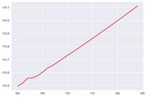
In H, we build the convolutional neural network model. In I, we train the model using the training data. In J, we use the model that we have trained to predict the next 24 values. These were the predictions when I ran the above Convolutional Neural Network python code:
>>> pred_Close
array([ 113.49421692,  113.51833344,  113.55593872,  113.55843353,
        113.57501984,  113.60240936,  113.63356018,  113.65409851,
        113.6788559 ,  113.70591736,  113.73150635,  113.75663757,
        113.78296661,  113.80939484,  113.83570099,  113.86231232,
        113.88925171,  113.91631317,  113.94355774,  113.97105408,
        113.99875641,  114.0266571 ,  114.05477905,  114.08312225,
        114.11167908], dtype=float32)
>>> pred_Close[-1]
114.11168
>>>
There were the predictions and next day after 24 hours USDJPY closed at 114.08. So the predictions are pretty accurate. So you can see this model can work. In K, I have plotted the original data and the predicted data. You saw the input closing price in the plot posted just above. In the plot below you can see the predicted USDJPY close price after 24 hours. You can see from the plot below that price increased rapidly almost in a straight line. Price seldom travels in a straight line though in reality.
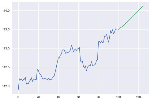
Now I have plotted USDJPY closing price and the predicted USDJPY closing price in the same plot just to make things more clear. Blue is the original closing price and green is the predicted price. There is an increase of almost 120 pips. We can build our trading strategy based on this deep learning model. When the model predicts price increase more than 100 pips in up or down direction, we open a trade accordingly in that direction with a profit target of 100 pips. Below is how this will look!
Convolutional Neural Network Algorithmic Trading System
Now that we have the basic convolutional network model that we will use to predict price after N bars which can be 10, 20, 30, 40. Too long a prediction horizon is not good. We will stick with a prediction horizon of N=24. This is what we will do. We will use H1 timeframe. At the end of every hour, we will make predictions for the next 24 hours. If our Convolutional Neural Network Model predicts a price move greater than 100 pips, we will open a trade in the direction of the prediction. If prediction is less than 100 pips, we will not open a trade. We will be using Oanda API. You can install OandapyV20 API. We will be using this OandapyV20 API to build a data streaming class. We can use this streaming class to predict price at the start of each new 60 minute candle. We can also choose 30 minute and 15 minute but in that case the prediction horizon becomes too large. But we can try that as on lower timeframe we detect the turning points much earlier.
I have a Daul core computer. On my computer this Convoltional Neural Network takes less than 30 minute to make the predicitons. I have bought a Quad Core computer with NVIDIA graphics card. On this computer, the model takes less than 20 seconds to make the predictions. So if you have a gaming computer meaning Quad Core with Graphics Card, you can use this model to trade on high frequency timeframes like 1 minute and even 30 seconds. If you don’t have a gaming computer you can still use this model to trade on M30, M60 and M240 timeframes.
One thing that I want to point out at this point is that I have used a regression Convolutional Neural Network Model on the closing price that uses MAE. We can also build a classification model that uses a different error function that uses entropy or something like that to build another model and check the accuracy of the predictions. Error function plays a large role in the model. Choosing the right error function can help a lot in building a good model. We can also use a customized error function.
I hope you have liked this post. Python is a powerful object oriented language that has emerged as a leader in machine learning, deep learning and artificial intelligence. There are many brokers who provide C# APIs for algorithmic trading. I have developed a few courses on how to use C# in algorithmic trading. The first course is C# for traders. In this course, I teach you the basics of C#. No previous programming experience is required. Once you master the basics of C#, you can take the second course C# Machine Learning For Traders. In this course I teach you how to do machine learning with C#. The last course is C# for Algorithmic Trading. Learning these languages Python and C# was fun for me. You too can easily learn these languages and build algorithmic trading systems using them with a little effort.