Trading is all about forecasting price. If you have been reading my Forex Strategies 2.0 Blog, you must have seen I am focusing more and more on algorithmic trading. If you can forecast currency pair price with a reasonable degree of accuracy, you can make a lot of pips. Markets have changed a lot. Today algorithms rule the market. Wall Street is being ruled by algorithmic trading systems. Big banks and hedge funds have developed their own algorithmic trading systems that don’t need any human intervention at all. Facebook Core Data Science Team released it’s Prophet for public in March of this year. Facebook has been using this algorithm extensively for making reliable forecasting for planning and goal setting. Prophet is a method for forecasting time series data. It is a robust algorithm which uses the standard General Additive Models to model non linear time series. Prophet can deal with missing data, big outliers and shifts in trends. When we are forecasting currency prices we are forecasting financial time series. Currency prices suddenly change direction meaning currency prices have lot of shits in trends. In this post I am going to discuss how we can use Facebook’s Prophet Algorithm in forex trading. Did you read the post that explains why high frequency returns are not normally distributed?
Facebook Prophet Algorithm is available in both R and Python. R and Python are two powerful machine learning languages that you should learn and master if you want to become an algorithmic trader. In this post we will be using R. Installing Prophet package is easy. Making forecasts with Prophet is pretty fast. Time taken is less than 1 second. This serves our purpose if we are trading high frequency data. Behind the scene this algorithm uses Stan. We don’t need to bother about Stan. Stan is used in Bayesian analysis. Using the algorithm in R is easy so don;’t worry at all what is Stan. First I want to discuss Prophet Algorithm in some detail so that we know how it models the time series. Prophet works best for daily data this is what the Core Data Science team says. So we will start off with daily data and in the end check if we can use this algorithm on high frequency data like 1 minute. Did you read the post on how to use Echo State Networks in forex trading?
Currency pair time series is known generally as financial time series. All financial markets have something in common. All financial markets are highly stochastic in nature and predicting a financial time series is a challenging task. A lot of research has been carried out but still it is very difficult to predict a financial time series. Let’s discuss GBPUSD daily time series. GBPUSD daily time series can change direction suddenly. We can break GBPUSD daily time series into 4 components:
- Growth function to model non periodic changes. For example FOMC Meeting announces rate hike. This suddenly forces GBPUSD daily price to soar high rapidly. We can model it as a growth function. Now you should keep this in mind, financial time series behaves differently when price rises and very differently when price falls. Price falls very rapidly as compared to when it rises. I think we can model this as a growth function.
- The second component that break the financial time series is the weekly seasonality. I don’t think we need to model monthly and yearly seasonality. We should keep Occam’s Razor that stipulates that we should keep the model as simple as possible.
- We need to have a model regarding holidays. Holidays can shock the market big time. As a currency trader I know a lot of things can happen over the weekend when the market is closed. On Sunday there can be some political statement that can move the market big time. For example, UK Prime Minister announced general elections over Sunday, On Monday, GBPUSD opened with a big gap. So we need to model the holidays as a separate component.
- An error term to model idiosyncratic changes that are missed by our model. We will assume that the error terms are normally distributed.
Sounds complicated? Good news! We don’t have to do anything. Prophet algorithm will do everything for us automatically. As said above, this algorithm uses Stan behind the scene which is a Bayesian algorithm. Everything is done automatically so we don’t have to worry a lot if we are getting good predictions. First we will let this algorithm make the prediction. If the prediction is not good, we can then tweak it to make the prediction more accurate. Let’s hope Prophet makes our life easy. We will have to check. Let’s start then. First read this post on a random walk with GBPUSD. In this post I show how we can use an auto-regressive model for predicting GBPUSD prices.
Keep this in mind. Forex trading is all about correctly predicting the price. You don’t need to be 100% accurate. If you can predict the market direction you can reduce your losing trades by 50%. In the past few years, trading has become very very algorithmic. Today algorithms rule the market. Below is the R code to implement the Prophet algorithm.
> library("prophet")
Loading required package: Rcpp
> library("readr")
> data <- read_csv("D:/MarketData/EURUSD+1440.csv",
+                  col_names=c("Date", "Time", "Open", "High",
+                              "Low", "Close", "Volume"),
+                  col_types=cols(Date=col_date(format='%Y.%m.%d')))
> x1 <-nrow(data)
> data <- data[, -2]
> data1 <- data[(x1-400):(x1-35),]
> df1 <- data1[, c(1,5)]
> head(df1)
# A tibble: 6 × 2
        Date   Close
      <date>   <dbl>
1 2015-11-10 1.07241
2 2015-11-11 1.07440
3 2015-11-12 1.08137
4 2015-11-13 1.07492
5 2015-11-16 1.06863
6 2015-11-17 1.06424
> tail(df1)
# A tibble: 6 × 2
        Date   Close
      <date>   <dbl>
1 2017-03-31 1.06581
2 2017-04-03 1.06686
3 2017-04-04 1.06725
4 2017-04-05 1.06625
5 2017-04-06 1.06435
6 2017-04-07 1.05958
> colnames(df1) <- c("ds", "y")
> m1 <- prophet(df1)
STAN OPTIMIZATION COMMAND (LBFGS)
init = user
save_iterations = 1
init_alpha = 0.001
tol_obj = 1e-012
tol_grad = 1e-008
tol_param = 1e-008
tol_rel_obj = 10000
tol_rel_grad = 1e+007
history_size = 5
seed = 291079117
initial log joint probability = -2.24128
Optimization terminated normally:
  Convergence detected: relative gradient magnitude is below tolerance
> str(m1)
List of 18
 $ growth                 : chr "linear"
 $ changepoints           : Date[1:25], format: "2015-11-26" "2015-12-11" "2015-12-30" ...
 $ n.changepoints         : num 25
 $ yearly.seasonality     : logi TRUE
 $ weekly.seasonality     : logi TRUE
 $ holidays               : NULL
 $ seasonality.prior.scale: num 10
 $ changepoint.prior.scale: num 0.05
 $ holidays.prior.scale   : num 10
 $ mcmc.samples           : num 0
 $ interval.width         : num 0.8
 $ uncertainty.samples    : num 1000
 $ start                  : Date[1:1], format: "2015-11-10"
 $ end                    : Date[1:1], format: "2017-04-07"
 $ y.scale                : num 1.15
 $ stan.fit               : NULL
 $ params                 :List of 6
  ..$ k        : num 0.24
  ..$ m        : num 0.947
  ..$ delta    : num [1, 1:25] -2.21e-08 -2.77e-01 -1.27e-01 1.14e-01 8.74e-02 ...
  ..$ sigma_obs: num 0.00647
  ..$ beta     : num [1, 1:27] 0 0.01132 -0.01187 0.00207 -0.00951 ...
  ..$ gamma    : num [1:25(1d)] 6.88e-10 1.67e-02 1.23e-02 -1.53e-02 -1.43e-02 ...
 $ history                :Classes ‘tbl_df’, ‘tbl’ and 'data.frame':	366 obs. of  4 variables:
  ..$ ds      : Date[1:366], format: "2015-11-10" "2015-11-11" "2015-11-12" ...
  ..$ y       : num [1:366] 1.07 1.07 1.08 1.07 1.07 ...
  ..$ t       : num [1:366] 0 0.00195 0.00389 0.00584 0.01167 ...
  ..$ y_scaled: num [1:366] 0.93 0.932 0.938 0.932 0.927 ...
 - attr(*, "class")= chr [1:2] "list" "prophet"
> future <- make_future_dataframe(m1, periods = 35)
> tail(future)
            ds
395 2017-05-06
396 2017-05-07
397 2017-05-08
398 2017-05-09
399 2017-05-10
400 2017-05-11
> forecast1 <- prophet:::predict.prophet(m1, future)
> plot(m1, forecast1)
> prophet_plot_components(m1, forecast1)
We have used the daily data. If you read the Facebook documentation for Prophet Algorithm, it says it works best for daily data. Now this algorithm makes the forecasting automatically. Take a plot of the forecast.
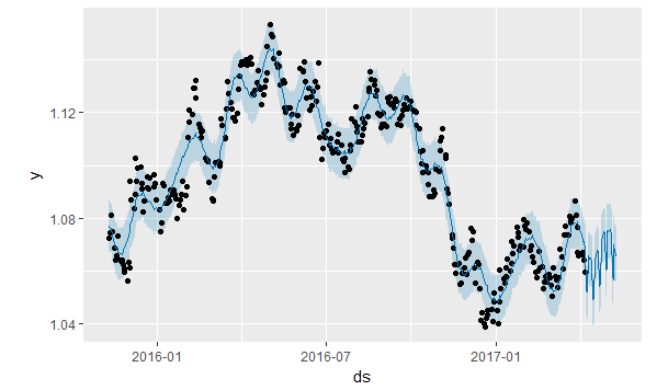
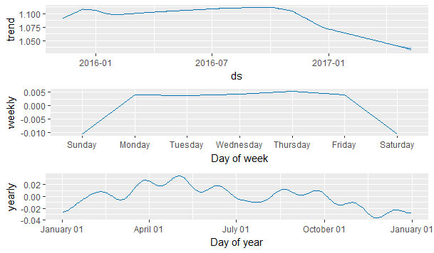
Above you can see the plot of the forecast with the tolerance levels. Prophet gives you the higher and lower tolerance levels of the forecast as well. We can also decompose the above plot into the trend, weekly seasonality and the yearly seasonality.
Below is the forecast made in tabular form.
> tail(forecast1, 35)
            ds        t    trend yhat_lower yhat_upper trend_lower trend_upper
366 2017-04-07 1.000000 1.043909   1.058503   1.078211    1.043909    1.043909
367 2017-04-08 1.001946 1.043621   1.043833   1.062444    1.043621    1.043621
368 2017-04-09 1.003891 1.043332   1.041914   1.061872    1.043332    1.043332
369 2017-04-10 1.005837 1.043043   1.055876   1.075024    1.043043    1.043043
370 2017-04-11 1.007782 1.042754   1.055409   1.073975    1.042754    1.042754
371 2017-04-12 1.009728 1.042465   1.054134   1.074271    1.042456    1.042487
372 2017-04-13 1.011673 1.042177   1.054888   1.074283    1.042117    1.042242
373 2017-04-14 1.013619 1.041888   1.054295   1.073646    1.041768    1.041996
374 2017-04-15 1.015564 1.041599   1.039399   1.058453    1.041402    1.041760
375 2017-04-16 1.017510 1.041310   1.039957   1.058645    1.041027    1.041526
376 2017-04-17 1.019455 1.041021   1.053857   1.073535    1.040673    1.041310
377 2017-04-18 1.021401 1.040732   1.054952   1.073676    1.040310    1.041081
378 2017-04-19 1.023346 1.040444   1.056506   1.075516    1.039928    1.040880
379 2017-04-20 1.025292 1.040155   1.058690   1.077451    1.039515    1.040668
380 2017-04-21 1.027237 1.039866   1.057339   1.076062    1.039111    1.040482
381 2017-04-22 1.029183 1.039577   1.044391   1.063794    1.038662    1.040306
382 2017-04-23 1.031128 1.039288   1.045823   1.065195    1.038245    1.040151
383 2017-04-24 1.033074 1.039000   1.061313   1.079502    1.037819    1.039990
384 2017-04-25 1.035019 1.038711   1.062002   1.081521    1.037425    1.039808
385 2017-04-26 1.036965 1.038422   1.063460   1.082672    1.037037    1.039641
386 2017-04-27 1.038911 1.038133   1.064560   1.084120    1.036612    1.039439
387 2017-04-28 1.040856 1.037844   1.064104   1.083570    1.036158    1.039263
388 2017-04-29 1.042802 1.037555   1.050387   1.070318    1.035691    1.039108
389 2017-04-30 1.044747 1.037267   1.050766   1.070905    1.035266    1.039004
390 2017-05-01 1.046693 1.036978   1.065699   1.085166    1.034845    1.038860
391 2017-05-02 1.048638 1.036689   1.065438   1.085964    1.034422    1.038690
392 2017-05-03 1.050584 1.036400   1.064749   1.085240    1.033968    1.038531
393 2017-05-04 1.052529 1.036111   1.065050   1.085800    1.033469    1.038364
394 2017-05-05 1.054475 1.035823   1.063513   1.083653    1.033025    1.038218
395 2017-05-06 1.056420 1.035534   1.048354   1.067641    1.032520    1.038083
396 2017-05-07 1.058366 1.035245   1.047477   1.066702    1.032109    1.037961
397 2017-05-08 1.060311 1.034956   1.058802   1.081033    1.031638    1.037860
398 2017-05-09 1.062257 1.034667   1.056254   1.078206    1.031123    1.037776
399 2017-05-10 1.064202 1.034379   1.056461   1.077099    1.030642    1.037677
400 2017-05-11 1.066148 1.034090   1.054501   1.076564    1.030145    1.037589
    seasonal_lower seasonal_upper       weekly weekly_lower weekly_upper     yearly
366    0.024767093    0.024767093  0.003940483  0.003940483  0.003940483 0.02082661
367    0.009575525    0.009575525 -0.010410964 -0.010410964 -0.010410964 0.01998649
368    0.008836971    0.008836971 -0.010410964 -0.010410964 -0.010410964 0.01924793
369    0.022674169    0.022674169  0.004035024  0.004035024  0.004035024 0.01863914
370    0.021769561    0.021769561  0.003585140  0.003585140  0.003585140 0.01818442
371    0.022019978    0.022019978  0.004116473  0.004116473  0.004116473 0.01790350
372    0.022955847    0.022955847  0.005144808  0.005144808  0.005144808 0.01781104
373    0.021856639    0.021856639  0.003940483  0.003940483  0.003940483 0.01791616
374    0.007811249    0.007811249 -0.010410964 -0.010410964 -0.010410964 0.01822221
375    0.008315721    0.008315721 -0.010410964 -0.010410964 -0.010410964 0.01872669
376    0.023456231    0.023456231  0.004035024  0.004035024  0.004035024 0.01942121
377    0.023876916    0.023876916  0.003585140  0.003585140  0.003585140 0.02029178
378    0.025435576    0.025435576  0.004116473  0.004116473  0.004116473 0.02131910
379    0.027623915    0.027623915  0.005144808  0.005144808  0.005144808 0.02247911
380    0.027684018    0.027684018  0.003940483  0.003940483  0.003940483 0.02374354
381    0.014669739    0.014669739 -0.010410964 -0.010410964 -0.010410964 0.02508070
382    0.016045356    0.016045356 -0.010410964 -0.010410964 -0.010410964 0.02645632
383    0.031869409    0.031869409  0.004035024  0.004035024  0.004035024 0.02783439
384    0.032763285    0.032763285  0.003585140  0.003585140  0.003585140 0.02917814
385    0.034567524    0.034567524  0.004116473  0.004116473  0.004116473 0.03045105
386    0.036762544    0.036762544  0.005144808  0.005144808  0.005144808 0.03161774
387    0.036585428    0.036585428  0.003940483  0.003940483  0.003940483 0.03264494
388    0.023091454    0.023091454 -0.010410964 -0.010410964 -0.010410964 0.03350242
389    0.023752733    0.023752733 -0.010410964 -0.010410964 -0.010410964 0.03416370
390    0.038641851    0.038641851  0.004035024  0.004035024  0.004035024 0.03460683
391    0.038400090    0.038400090  0.003585140  0.003585140  0.003585140 0.03481495
392    0.038893224    0.038893224  0.004116473  0.004116473  0.004116473 0.03477675
393    0.039631580    0.039631580  0.005144808  0.005144808  0.005144808 0.03448677
394    0.037886050    0.037886050  0.003940483  0.003940483  0.003940483 0.03394557
395    0.022748729    0.022748729 -0.010410964 -0.010410964 -0.010410964 0.03315969
396    0.021730599    0.021730599 -0.010410964 -0.010410964 -0.010410964 0.03214156
397    0.034944144    0.034944144  0.004035024  0.004035024  0.004035024 0.03090912
398    0.033070537    0.033070537  0.003585140  0.003585140  0.003585140 0.02948540
399    0.032014391    0.032014391  0.004116473  0.004116473  0.004116473 0.02789792
400    0.031322816    0.031322816  0.005144808  0.005144808  0.005144808 0.02617801
    yearly_lower yearly_upper    seasonal     yhat
366   0.02082661   0.02082661 0.024767093 1.068676
367   0.01998649   0.01998649 0.009575525 1.053196
368   0.01924793   0.01924793 0.008836971 1.052169
369   0.01863914   0.01863914 0.022674169 1.065717
370   0.01818442   0.01818442 0.021769561 1.064524
371   0.01790350   0.01790350 0.022019978 1.064485
372   0.01781104   0.01781104 0.022955847 1.065132
373   0.01791616   0.01791616 0.021856639 1.063744
374   0.01822221   0.01822221 0.007811249 1.049410
375   0.01872669   0.01872669 0.008315721 1.049626
376   0.01942121   0.01942121 0.023456231 1.064477
377   0.02029178   0.02029178 0.023876916 1.064609
378   0.02131910   0.02131910 0.025435576 1.065879
379   0.02247911   0.02247911 0.027623915 1.067779
380   0.02374354   0.02374354 0.027684018 1.067550
381   0.02508070   0.02508070 0.014669739 1.054247
382   0.02645632   0.02645632 0.016045356 1.055334
383   0.02783439   0.02783439 0.031869409 1.070869
384   0.02917814   0.02917814 0.032763285 1.071474
385   0.03045105   0.03045105 0.034567524 1.072989
386   0.03161774   0.03161774 0.036762544 1.074896
387   0.03264494   0.03264494 0.036585428 1.074430
388   0.03350242   0.03350242 0.023091454 1.060647
389   0.03416370   0.03416370 0.023752733 1.061019
390   0.03460683   0.03460683 0.038641851 1.075620
391   0.03481495   0.03481495 0.038400090 1.075089
392   0.03477675   0.03477675 0.038893224 1.075293
393   0.03448677   0.03448677 0.039631580 1.075743
394   0.03394557   0.03394557 0.037886050 1.073709
395   0.03315969   0.03315969 0.022748729 1.058283
396   0.03214156   0.03214156 0.021730599 1.056976
397   0.03090912   0.03090912 0.034944144 1.069900
398   0.02948540   0.02948540 0.033070537 1.067738
399   0.02789792   0.02789792 0.032014391 1.066393
400   0.02617801   0.02617801 0.031322816 1.065413
Above was the forecast made by Facebook Prophet algorithm. Actual daily closes prices are below.
> tail(data, 35)
# A tibble: 35 × 6
         Date    Open    High     Low   Close Volume
       <date>   <dbl>   <dbl>   <dbl>   <dbl>  <int>
1  2017-04-10 1.05881 1.06060 1.05690 1.05953 143236
2  2017-04-11 1.05950 1.06292 1.05778 1.06036 160464
3  2017-04-12 1.06038 1.06742 1.05881 1.06634 177756
4  2017-04-13 1.06626 1.06768 1.06083 1.06133 170756
5  2017-04-14 1.06155 1.06290 1.06052 1.06106  93307
6  2017-04-17 1.06040 1.06697 1.06036 1.06425  61564
7  2017-04-18 1.06417 1.07353 1.06365 1.07294 121388
8  2017-04-19 1.07297 1.07363 1.06990 1.07109  95794
9  2017-04-20 1.07129 1.07768 1.07084 1.07167 101258
10 2017-04-21 1.07159 1.07373 1.06815 1.07068  96497
# ... with 25 more rows
You can compare the predictions with the actual. As said above, if we can predict the market direction correctly, we can use it in our trading strategy to reduce more than 50% of the losing trades. It maybe impossible to predict the price correctly. We should focus more on the market direction. Read the post in which I explain how you can get a free forex VPS on Amazon Web Services.