In this post we are going to apply the random walk model to GBPUSD pair. We will check whether the standard random walk model as being taught in most time series analysis textbooks can help in improving our forex strategy. Before you continue did you read the post on how to read the charts? If you haven’t you should it is a good post that contains a 60 minute video on how to trade charts. Just by looking at the charts, you can understand what the market is doing and what it will most probably do. We look at charts and try to identify chart patterns that we believe can tell us where the market will be going in near future. This is known as Technical Analysis.
Technical Analysis Versus Statistical Analysis
Technical analysis is based on the thinking that past price has information about the near term future price. Now most of us technical traders use bar patterns and candlestick patterns when we do technical analysis. We believe that there are certain high probability candlestick patterns as well as bar patterns that tell us when the market is going to change the trend direction and continue in the direction of the trend. These patterns are known as trend reversal patterns as well as trend continuation patterns. In simple terms what we are doing is looking at the past 5-10 candles on the charts and looking for our favorite patterns. When we have a pattern identified we use them to predict the future market direction.
Did you read the post on how to master trading psychology and overcome fear and greed in trading? How do fear and greed develop in trading? This is an important question that we need to address now. When we are trading on our whims and wishes we are giving full control to our emotions of fear and greed. When we lose we become fearful. So we avoid to trade when we have a good setup. In the same manner when we win we tend to become greedy and we think we can open a new trade even when the trade setup is not confirmed. The only way to master trading psychology is by having a trading system that is rule based and has been tested thoroughly. Having said that, you should now understand why we need a solid trading system.
As said above Technical Analysis is based on the premise that past price can be used to predict the near term future price. Now we will do the same thing but in a different manner in this post with the tools used in Statistical Analysis. This premise that the past holds the secret to predict the future is also being used in statistical analysis tool of time series. Past values of a time series are serially correlated and have important information that we can use to predict the near term future values of that time series. So let’s discuss time series and how we can use them in trading GBPUSD and for that matter any other currency pair.
Time Series Analysis And Stochastic Trends
Time series are variables measured sequentially in time. Time series appear frequently in different branches of science, engineering and commerce. Global warming was proved with the help of time series analysis. So you can well imagine how much developed this statistical analysis tool has become over the past few decades. Each time series is composes of trends which can be deterministic or stochastic. In addition to that there are seasonal variations as well as other cyclical variations. The video below explains the difference between deterministic and stochastic trends.
Now let’s focus on the currency market. Price data for each pair like GBPUSD, EURUSD, NZDUSD, USDJPY etc is available down to the 1 minute level. We can even go below the 1 minute level. When price changes it is recorded as a Tick. Tick data is also available. We are living in the age of Big Data. Data Science is a new field of study that studies data and tries to extract meaningful actionable information out of it. In forex the field which we are discussing most of the time price gets updated after every few seconds something like 1-10 seconds. So every 1-10 seconds we receive a tick on our MT4 platform. MT4 platform then converts those ticks into Open, High, Low and Close for each time interval.
If we want to download price data we can download 1 minute, 5 minute 15 minute, 30 minute, 1 hour, 4 hour, daily, weekly and monthly data. This data comprises of Open, High, Low and Close and Volume for that time interval. So the data that we have is already in the shape of a time series as it has been measure sequentially. We now need to just analyze it statistically using time series analysis methods and see if we can extract some meaningful information out of it that can help us in taking better trading decisions.
Now as said above time series data comprises of trends which can be deterministic or stochastic. Deterministic trend develops when we can use some physical law to measure it. For example if the trend increases with time, we can use time to model it. Once we know the physical law describing the trend, we can then predict it in the future as well as long as that physical law governing that trend does not changes. But the trends that get developed in the currency market change directions often and have no physical laws behind them. That’s why they are known as Stochastic Trends. We will be dealing with Stochastic Trends. It is difficult to predict Stochastic Trends. The best we can do is predict the trend ahead a few steps. There is always a possibility that the trend changes direction and we have our predictions wrong. So it is always difficult to predict stochastic trends in the future.
Open Source Powerful Data Science Software R
We will be using this powerful open source data science software R. R software can be download FREE. But before you can use it you will need to learn R language. R language is not difficult to learn. Once you have learned this language you will be able to use more than 2500+ statistical and machine learning algorithm packages that have been developed by the R community. The data can be easily converted into a time series object and then we can use the different time series packages that are available. So let’s start our time series modelling of GBPUSD data. First download GBPUSD weekly, daily, H4, H1, M30, M15, M5 and M1 data as csv files. You can easily do that. Open MT4 Tools > History Center > GBPUSD.
Random Walk Model of GBPUSD
We will develop a Random Walk model of GBPUSD in this post and check if we can use it in our trading. Random walk is a model that is often used in statistical analysis of a time series. Watch the video below that explains what a random walk model is:
Now having viewed above video, you should be clear what a random walk model is. So let’s start.
> # Import the csv file
> quotes <- read.csv("E:/MarketData/GBPUSD10080.csv", header=FALSE)
> #convert the data frame into an xts object
> quotes1 <- as.ts(quotes)
> class(quotes1)
[1] "mts"    "ts"     "matrix"
> tail(quotes1)
          V1 V2      V3      V4      V5      V6      V7
[1072,] 1072  1 1.44625 1.46609 1.41805 1.42742  648469
[1073,] 1073  1 1.42680 1.43881 1.40127 1.43604  716947
[1074,] 1074  1 1.44729 1.50135 1.32223 1.36770 1045560
[1075,] 1075  1 1.34245 1.35340 1.31211 1.32730  880883
[1076,] 1076  1 1.32501 1.33416 1.27974 1.29493  665168
[1077,] 1077  1 1.29514 1.34791 1.28507 1.33027  569945
> plot(quotes1[,6], xlab = "time/weeks",
+ ylab = "GBP/USD Weekly Close")
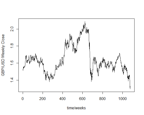
Above is the plot of the GBPUSD Weekly Close data for the many years, As you can see from above there are around 1074 closing prices available in our data. You can see in the above plot first there was a strong appreciation of GBPUSD exchange rate then there was a strong depreciation of GBPUSD exchange rate. After that in the last few weeks you can see the after shocks caused by Brexit.
Checking The GBPUSD Exchange Rate Weekly Time Series For Stationarity
Stationarity is an important condition. Stationarity means that the mean of the time series does not changes with time. Just looking at the above time series plot we can see that the mean of this time series is changing with time. So the above GBPUSD exchange rate time series does not satisfy the stationarity condition. If you are not still not sure what this stationary condition means, you can watch this video that explains what stationary means for a time series:
The video below explains the difference between stationary and non stationary time series.
In the plot below we show the correlogram of the GBPUSD weekly close time series.
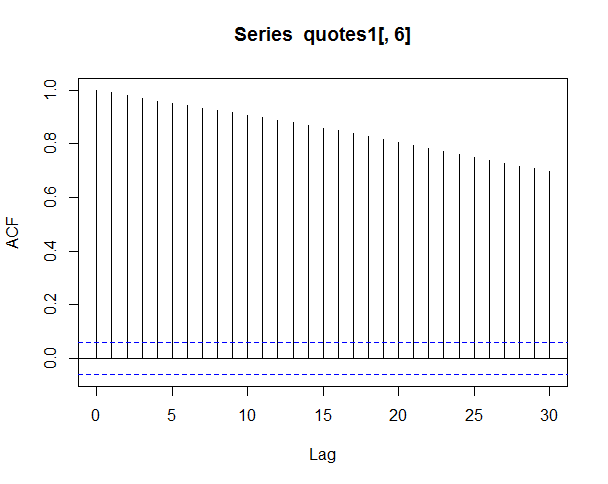
Above is the Correlogram of GBPUSD Weekly Close time series. Above correlogram is the plot of the Auto Correlation Function of the weekly close series. The above plot shows that the different values are serially correlated with its near past values. If you are not sure what serial correlation means, you can watch this video that explains what serial correlation means:
In nutshell serial correlation means that the past values have correlations with the present value. This is an indications that the past holds information about the present. How do we deal with serial correlation? In order to extract the information that is contained in serial correlation, we need to convert the above time series in such a manner so that the residuals is just white noise. If we take the logarithm of the close price and then difference it we get the weekly returns series that has residuals which are white noise. This will become apparent when we draw its correlogram.
> #calculate log returns
> lr <- diff(log(quotes1))
> acf (lr[,6])
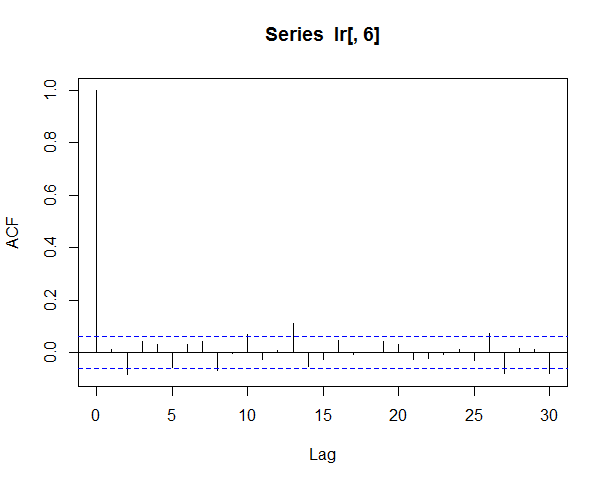
Above is the correlogram of log difference of the weekly close price. You can see that the above correlogram is drastically different from the previous correlogram. In the above correlogram you can see that the all auto correlations are below the 0.05 level which is a good indication that the residuals of the log of the weekly close price is a white noise. Now let’s fit an autogression model to the above time series of log difference of the weekly close price which is very close of the weekly returns of the GBPUSD using the Akaike Information Criterion. You can watch the video below that explains Akaike Information Criterion (AIC):
Now let’s fit a random walk model and check if we get good results and can we use it in trading. Below are the results of the calculations made by R:
> # Import the csv file
> quotes <- read.csv("E:/MarketData/GBPUSD10080.csv", header=FALSE)
>
>
> #convert the data frame into an xts object
> quotes1 <- as.ts(quotes)
>
> class(quotes1)
[1] "mts"    "ts"     "matrix"
>
> tail(quotes1)
          V1 V2      V3      V4      V5      V6      V7
[1072,] 1072  1 1.44625 1.46609 1.41805 1.42742  648469
[1073,] 1073  1 1.42680 1.43881 1.40127 1.43604  716947
[1074,] 1074  1 1.44729 1.50135 1.32223 1.36770 1045560
[1075,] 1075  1 1.34245 1.35340 1.31211 1.32730  880883
[1076,] 1076  1 1.32501 1.33416 1.27974 1.29493  665168
[1077,] 1077  1 1.29514 1.34791 1.28507 1.33027  569945
>
>
> plot(quotes1[,6], xlab = "time/weeks",
+      ylab = "GBP/USD Weekly Close")
>
> acf (quotes1[,6])
>
>
>
> #calculate log returns
>
> lr <- log(quotes1)
>
>
>
> acf (lr[,6])
>
> lr1 <- ts(lr, start=1, end=1000)
>
> lr1[990:1000,6]
 [1] 0.4491757 0.4480839 0.4458070 0.4432874 0.4521706 0.4466198 0.4416942 0.4275201 0.4163259
[10] 0.4158510 0.4049383
> lr[990:1000,6]
 [1] 0.4491757 0.4480839 0.4458070 0.4432874 0.4521706 0.4466198 0.4416942 0.4275201 0.4163259
[10] 0.4158510 0.4049383
>
> model <- ar(lr1[,6], aic=TRUE, method='mle')
> model

Call:
ar(x = lr1[, 6], aic = TRUE, method = "mle")

Coefficients:
      1        2        3        4        5        6        7        8        9       10
 1.0097  -0.0827   0.1280  -0.0506  -0.0413   0.0502   0.0182  -0.1032   0.0802   0.0522
     11
-0.0704

Order selected 11  sigma^2 estimated as  0.0001461
> predict(model, n.ahead = 20)
$pred
Time Series:
Start = 1001
End = 1020
Frequency = 1
 [1] 0.4051536 0.4058552 0.4061479 0.4068694 0.4080298 0.4087311 0.4079629 0.4087702 0.4095433
[10] 0.4095259 0.4104342 0.4114693 0.4122428 0.4130877 0.4141630 0.4150111 0.4157456 0.4167085
[19] 0.4175853 0.4183648

$se
Time Series:
Start = 1001
End = 1020
Frequency = 1
 [1] 0.01208694 0.01717685 0.02057373 0.02380380 0.02670406 0.02910017 0.03137814 0.03366780
 [9] 0.03550333 0.03725884 0.03921663 0.04101719 0.04266397 0.04427078 0.04579272 0.04719973
[17] 0.04856583 0.04988414 0.05110876 0.05228603

>
> lr[1001:1020,6]
 [1] 0.4104991 0.4214762 0.4316071 0.4313797 0.4343052 0.4083742 0.3884478 0.4021864 0.3979100
[10] 0.3985882 0.3807215 0.4027815 0.4176440 0.4160291 0.4354769 0.4527812 0.4370348 0.4244504
[19] 0.4236913 0.4425939
In the last 3 paras you can compare the predicted results of the auto regression model. The first predicted value of the log normal price is 0.4051 whereas the actual log normal price is 0.4104. So what to do? Our autogressive model is underestimating the first prediction and the later predictions are wide off the mark. The above post is a clear indication that we cannot trade GBPUSD based on the random walk model. The predictions are not good. In the next post we try exponential smoothing and the Hold Winters method and check if we can good predictions. Did you read the post on a swing trade that made 270% in 1 week?